Portable Partial Discharge Detector: Four Sensors That Do Not Measure the Same Thing

A technician clamps an HFCT around the earth strap of a 10 kV switchgear cubicle, presses the probe against the front panel, and the portable partial discharge detector returns four numbers: a transient earth voltage in dB, an airborne ultrasonic level in dBµV, a high-frequency current in pC, and a UHF level in dBm.

Below them, one colour bar.

Three of those four are not charges. None of them shares a unit with the others. And the bar is a heuristic the instrument applies across four physically different observations - which is why it works as a screening tool and why it must never be written into a test report as though it were a result.

The four channels are usually presented as four ways to find the same defect. They are better understood as four different physical measurements that happen to respond to the same event.

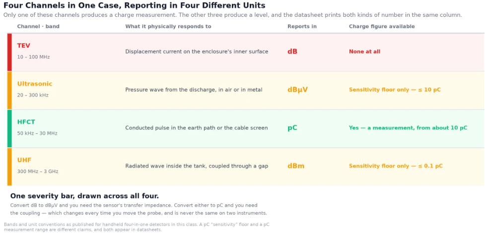
Figure 1 - The unit column is the one to read. HFCT is the only channel that produces a charge; the other three produce a level whose reference lives inside the instrument.

TEV reads the displacement current that a discharge drives onto the inner surface of an earthed metal enclosure. It is a genuinely useful screening channel on metal-clad switchgear, and it reports in dB - a level, referenced to whatever the probe and its front end produce for a given field. There is no charge in that number, and no way to put one there without knowing the enclosure's transfer behaviour.

Ultrasonic reads a pressure wave, in dBµV, relative to a microphone sensitivity convention. What it measures depends on whether the wave reached it through air or through metal, and on how far it travelled.

HFCT reads a conducted pulse in the earth path or the cable screen, across a known impedance, and that is what makes a charge figure possible at all. It is the only channel of the four where pC is an honest unit rather than a convenience.

UHF reads a radiated wave that has escaped the enclosure through some aperture. The reading in dBm depends on the aperture, which is why UHF is excellent on GIS with a designed coupler and unreliable on switchgear with none.

The tell is in the datasheets. A four-in-one instrument in this class will typically claim ≤ 0.1 pC on UHF, ≤ 5 pC on HF and ≤ 10 pC on acoustic - a hundredfold spread across three channels of one instrument. Those are not three measurements on a common scale. Each was obtained by a different conversion from a different physical quantity, and the numbers land in the same column of the table because the table has one column for them.

A pC sensitivity floor and a pC measurement are different claims. The first says "below this, I cannot see it." The second says "this is what it is." Only one channel supports the second.

The ultrasonic channel has a second problem, and this one is arithmetic rather than convention.

Sound pressure in a free field falls as 1/r. In decibels that is 20 dB per decade of distance: move the probe from 10 cm to 1 m and the reading drops 20 dB, which on a typical 0–60 dB scale is a third of the instrument's entire range.

Figure 2 - Two parallel curves. Moving the probe and weakening the defect trade against each other exactly, so no single reading can say which one moved.

Now the consequence, which is exact rather than approximate. If the defect is ten times weaker and the probe is ten times closer, the pressure at the microphone is identical. A defect ten times weaker at 10 cm reads exactly the same as a defect ten times stronger at 1 m.

So the airborne ultrasonic channel measures severity and geometry in the same number, and offers no way to separate them. A survey that ranks cubicles by the loudest ultrasonic reading is ranking them by a combination of defect size and how close the technician happened to stand.

Two things follow, and both are practical.

Prefer the contact channel for comparison. A contact acoustic sensor coupled to a defined point on the panel removes the distance variable, which is why the same instrument's contact and airborne modes should not be treated as interchangeable readings.

Never compare airborne readings taken from different distances. If a survey procedure says "point the probe at the panel", it has already given up the ability to compare one cubicle with another. Fix the distance, or accept that the numbers are local.

The same logic applies, less severely, to TEV. The signal travels on the enclosure's inner surface and attenuates at panel joints, gaskets and paint. A probe on a painted cover reads low not because the defect is small but because the path is long - and a defect behind a barrier may not be visible at all.

There is a third trap, and it is in the reader rather than the instrument.

Decibels are a ratio, not a quantity. 6 dB is a factor of two. 20 dB is a factor of ten. An operator who sees 36 dB on one cubicle and 30 dB on the next perceives a difference of six "units" and mentally files it as a modest variation. It is a factor of two.

Across a 60 dB instrument range, the span from bottom to top is a factor of one thousand in amplitude. The difference between "worth noting" and "open the panel" can be a handful of dB, and the eye does not weight it correctly.

The practical fix costs nothing: when a threshold is set in dB, write the corresponding ratio beside it in the method statement. "Alarm at 40 dB, twice the typical background of 34 dB" is a statement an engineer can sanity-check. "Alarm at 40 dB" is a number someone will argue with for an hour.

The pattern is the diagnosis. The number is a screening index

Here is the part that gets undersold in the marketing, because it is harder to put on a feature list.

The reason a portable detector beats a passive indicator is not the sensitivity figure. It is the phase-resolved display. Real partial discharge is locked to the power-frequency cycle, so its pulses cluster at characteristic phase positions and form a recognisable shape. Switching noise from a neighbouring drive is not locked to that cycle, so it scatters.

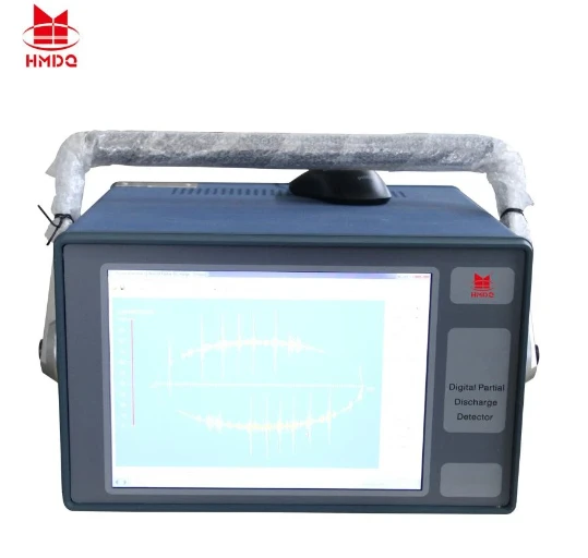
Figure 3 - The display is the instrument. A two-lobed pattern locked to the phase axis is a different class of evidence from a number, because it separates a discharge inside the insulation from the electrical noise around it.

That difference is what lets an experienced operator say "that is internal discharge in the busbar insulation" rather than "something is at 42 dB". It is also the layer that IEC TS 62478 addresses when it treats electromagnetic and acoustic methods as requiring their own location and sensitivity checks - the standard expects a response check per method, not one check for the box.

Three demonstrations get conflated in the field, and it is worth keeping them apart: a power-on check proves the instrument boots, a sensitivity check proves the signal path responds to a known pulse, and a diagnosis says what the insulation is doing. Passing the first two says nothing about the third.

Two words get used interchangeably here and they are not the same thing - which matters, because one is possible in a substation and the other is not.

Calibration, in the IEC 60270 sense, assigns a pC value. A known charge is injected into a defined measuring circuit and the scale is set so that the reading corresponds to it. That requires the circuit. A handheld probe pressed against a switchgear panel has no defined circuit, so there is nothing to calibrate against - and any instrument claiming a calibrated pC reading in that configuration is claiming something the physics will not support.

A sensitivity check asks a weaker and answerable question: does this chain - sensor, cable, front end, software - respond to a stimulus of a defined kind? IEC TS 62478 treats this as a per-method requirement, and the per-method part is what people skip. A check that proves the acoustic path says nothing whatever about the UHF one, so four channels need four checks.

What the check buys is a floor for belief. If the chain responds to a known pulse at the start of the survey, you know the readings that follow came from an instrument that was working. If it does not respond, you have found out before anything was written down rather than after.

What it does not buy is a conversion factor. A passed sensitivity check does not turn the subsequent dB figure into a charge, and it does not make two instruments comparable. It establishes that the number is reproducible on this unit - which, as the earlier sections argued, is the only thing the number was ever good for.

Four limits, all of them structural rather than defects in any particular product.

It cannot give you a pC figure traceable to IEC 60270. That standard calibrates a measurement by injecting a known charge into a defined circuit. In a live substation with a handheld probe there is no defined circuit and no injection point, so the reading is an index, not a measurement.

It cannot separate severity from geometry on the airborne channel. Twenty decibels per decade, as above.

It cannot be compared against a different make of instrument. Different front ends, different bandwidths, different reference levels - the dB figure from one unit is not the dB figure from another, and no conversion factor exists.

It cannot see a defect that is not active while you are looking. A portable detector applies whatever voltage the system happens to be at. A defect with an inception voltage above the operating point is silent, and will stay silent until a switching surge or a load change wakes it.

Goldhome's portable range covers the four channels in one handheld: acoustic emission across 10–300 kHz with a claimed sensitivity of ≤ 10 pC, UHF across 300–1500 MHz at ≤ 0.1 pC, high frequency across 3–30 MHz at ≤ 5 pC, and a TEV channel reported in dB. Sampling runs at 16 bit with 10 MS/s on the acoustic channels and 250 MS/s on UHF; the unit runs Windows CE on a roughly 1.5 kg body, and synchronises either from an external AC source of 10–380 V or wirelessly.

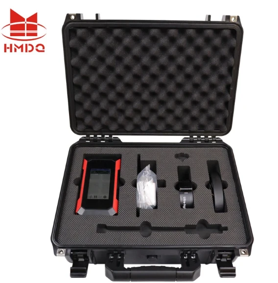
Figure 4 - Four sensor types, one case. The instrument is the small part; the case is what decides whether the survey is repeatable, because the coupling arrangement for each sensor is fixed by what is actually in those cut-outs.

Pages: partial discharge detectors · partial discharge tester · PD detection device · handheld ultrasonic PD detector · switchgear PD detection · full PD test equipment range.