In a Refinery, a PD Monitor Is Judged on Lead Time, Not Sensitivity

 An SITC scope for online partial discharge monitoring on a 220/33 kV, 65 MVA transformer ends at commissioning. Whether the system is still believed in year three is decided by one number that is not in the specification.

Take the asset first, because its numbers set the whole problem.

A 220/33 kV, 65 MVA transformer draws 171 A on the high-voltage side and 1 137 A on the 33 kV side. In a refinery that 33 kV winding almost certainly feeds large motor drives, which means the substation contains, by design, switching sources with nanosecond edges - the same rise time as the discharge the monitoring system is being bought to detect. The transformer is oil-immersed, the HV winding carries the highest dielectric stress, and the 33 kV side is most likely cable- or busduct-connected rather than overhead.

Now the consequence of a failure. A replacement at this rating and voltage class is a long-lead item, quoted in months. The refinery's own outage cost is measured in production, not in the transformer. And the maintenance calendar for a plant like this is set years in advance - a turnaround every four or five years, with the work packages frozen long before the unit comes down.

That last fact is the one that reframes the specification. If the monitoring system produces a warning six months before failure, the repair becomes a work package in a scheduled turnaround, priced and resourced like everything else. If it produces a warning six hours before failure, the refinery has exactly the emergency it would have had without the monitor, plus the invoice.

So the deliverable is not sensitivity. It is lead time. And lead time is not a property of the sensor. It is a property of the sensor and the site.

The case for permanent monitoring over periodic testing is the shape of the failure. PD from voids, moisture, contamination and mechanical damage develops over months. A periodic survey samples that curve at intervals and can miss it entirely; a permanent installation records the curve. For an asset that cannot be taken out at will, that is the whole argument.

It is worth being equally clear about the limits, because they determine what the system may be used to claim.

The applied voltage cannot be controlled. Offline, you know the voltage at which a defect incepts and extinguishes. Online, the transformer is at whatever the system needs it to be, and a defect that is inactive at that operating point will not appear.

Noise is present, and it is not an anomaly - it is the normal condition. Every method below is really a discrimination method.

Localisation and classification are harder. A pattern that would be unambiguous in a screened laboratory has to be separated from a site whose background is itself phase-resolved and structured.

Results are not comparable between assets. Two transformers with different sensor arrangements, different valve positions and different tank geometry do not produce comparable pC figures. A trend is valid on one asset; a league table across a fleet is not.

The distinction that matters commercially: an online system is excellent at trend and presence, and unreliable at absolute level. That is not a defect. It just has to be designed and reported as what it is.

Here is the arithmetic that decides the project, and it can be done on one sheet of paper before anything is ordered.

Every alarm threshold has to sit above the noise floor - otherwise the system alarms on the site. A reasonable commissioning choice is a threshold at about twice the measured floor. Which means the floor alone sets how early the first credible alarm can possibly arrive.

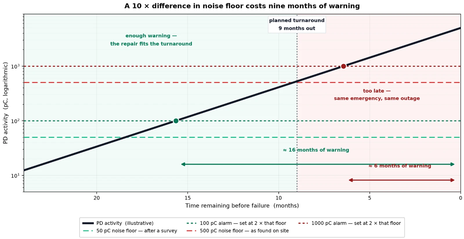
Figure 1 - The same transformer, the same defect, the same instrument. The only difference is the noise floor the system was commissioned against.

Run the two cases. A site surveyed properly before installation, with sensors placed where the background is lowest, might establish a floor around 50 pC and therefore an alarm at 100 pC. The same transformer, installed as-found with sensors wherever they were convenient and a floor around 500 pC, gets an alarm at 1 000 pC.

On the illustrative trend in Figure 1, the first crosses the alarm threshold about 16 months out. The second crosses about 6 months out - past a turnaround that was planned nine months ahead.

A factor of ten in the noise floor, and a difference of roughly nine months in warning. One of those systems produces a work package; the other produces a phone call at 02:00.

This is why the site survey is not a formality. It is the step that determines the project's outcome, and it is the step most often skipped because the tender already specified a sensitivity in pC and everyone assumed the specification was the hard part.

The second constraint is physical and cannot be engineered around: the sensor set is limited by the access points the transformer actually has.

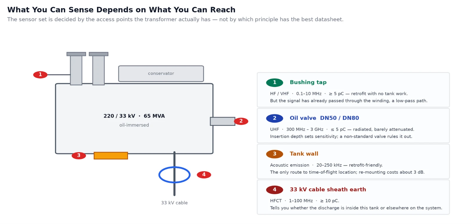
Figure 2 - Four routes in, four different views of the same tank. GB/T 42287-2022, identical to IEC TS 62478:2016, covers the electromagnetic and acoustic methods.

① The bushing tap gives a conducted signal path out of the transformer with no tank work at all, which makes it the most retrofit-friendly option on a 220 kV unit. The active band is roughly 0.1–10 MHz, and the sensor is an HFCT or a measuring impedance on the tap. But there is a physical catch worth understanding, because it explains why one sensor type is never enough: a discharge deep in the winding generates a fast pulse, yet the spectral content of the conducted signal falls to below a few megahertz after it has travelled through the winding, which behaves as a low-pass filter. The bushing tap sees what survives the winding.

② A UHF antenna in the oil valve sees something different. The radiated component escapes through the oil and reaches a sensor inserted through a standard DN50 or DN80 valve with only moderate attenuation, in the 300 MHz – 3 GHz band. Because the tank is a grounded steel enclosure, this sensor sits inside a Faraday cage - which is why UHF is the most interference-immune option available. Two constraints come with it: the insertion depth has a decisive influence on sensitivity, insertion is limited to protect the active part, and if the transformer does not have standardised oil valves, or invasive access is not permitted, the method is simply unavailable.

③ Acoustic emission sensors on the tank wall, in the 20–250 kHz band, are easy to retrofit and are the only route to time-of-flight localisation. They also carry a commissioning discipline: re-mounting a fixed acoustic sensor introduces a sensitivity deviation of roughly 3 dB, so placement should be planned once rather than adjusted by trial.

④ An HFCT on the 33 kV cable sheath earth. On a cable-connected transformer this sensor answers the single most useful question in the whole exercise: is the discharge inside this tank, or somewhere else on the 33 kV system? Given that the 33 kV side of a refinery substation is where the switching noise lives, that discrimination is worth more than several decibels of sensitivity.

Used together, electromagnetic and acoustic timing gives location: the error is the arrival-time difference multiplied by the acoustic velocity in oil - about 1 300 m/s at 50 °C. Reported results on transformers put the combined method at roughly ± 30 cm, which is the difference between "there is PD in this transformer" and "there is PD at the tap changer."

In a screened test bay, a PD measurement is a measurement. Here it is a separation problem, and the separation has to work against a background that is neither random nor benign.

Three classes of interference dominate:

Power-frequency-locked noise - corona on the 220 kV busbar, connections and hardware. From a signal-processing point of view this is genuine discharge activity; it is simply not inside the transformer. It is phase-locked to the supply, so it produces a clean and stable phase-resolved pattern, which is exactly what makes it dangerous: it looks like a finding.

Non-synchronised switching noise - the drives, rectifiers and converters on the 33 kV system. Their edges are fast enough to be indistinguishable from PD in the time domain, but they are not locked to the supply, so their pulses scatter across the phase axis rather than clustering.

Ambient radio and communications - FM, TV, GSM, Wi-Fi. This is the one class that a UHF sensor in the tank largely eliminates by construction.

Against that background, four discrimination tools do the work, and the experienced practice is to require several of them before believing anything:

Phase-resolved pattern analysis (PRPD / PRPS). Real internal discharge clusters at characteristic phase positions. Unsynchronised noise does not.

Coincidence across independent sensors, with a consistent arrival-time difference. A discharge inside the tank is seen by more than one sensor, with a delay that matches the internal path. External interference usually is not.

Frequency-band selection. The winding-limited bushing-tap path and the radiated UHF path are looking at different parts of the physics. A signal present in one and absent in the other is informative in itself.

Correlation with load and top-oil temperature. A rise that tracks load may be benign; a rise that does not is not.

Which leads to the design rule that matters most on a site like this:

No alarm without agreement between two independent sensing principles.

Not two sensors of the same type - two different principles. On a refinery substation this is not conservatism; it is the only configuration in which the alarm rate stays low enough for the alarms to keep being read. And it is worth asking the uncomfortable question during design rather than after: what would make a night-shift operator stop trusting this system? The answer is almost always a documented history of alarms that correlated with nothing.

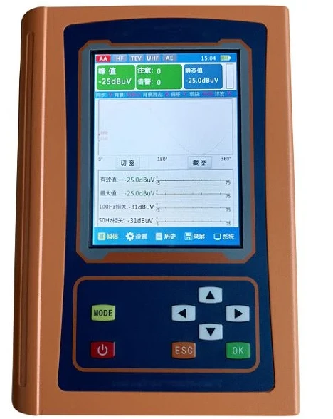
Figure 3 - The phase axis is the discriminator. This is the screen that decides whether a pulse belongs to the transformer or to the plant around it.

Stage 1 - Survey the site before you specify the system

The noise floor cannot be read off a datasheet and cannot be estimated from another substation. It has to be measured, on this transformer, at the actual sensor positions, with the unit in service.

A portable detector with a full sensor set is the right instrument for this stage: it can establish the band-by-band background at each candidate access point, capture the site's own phase-resolved signature so that "site normal" is a recorded reference rather than an assumption, and separate what is phase-locked from what is not.

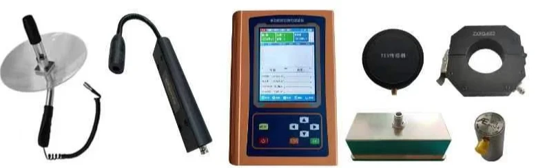
Figure 4 - The survey kit. Deliberately the same sensor families as the permanent installation, because the point of the survey is to predict what the permanent sensors will see.

The output of Stage 1 is a number per sensor position. Every threshold, every sensor choice and the achievable warning time follow from it. A project that skips this stage has bought a specification instead of a result.

Stage 2 - Choose sensors against the access, not the datasheet

Walk the list in Figure 2 against what the transformer actually offers. Bushing taps present? Oil valves standard, and is invasive access permitted? Is there an outage window for tank-wall work, or does everything have to be clamp-mounted? Is the 33 kV side cable-connected, making a sheath-earth HFCT available?

Then re-read Stage 1's numbers. A sensor that is theoretically more sensitive but sits where the site background is 400 pC is worse than a less sensitive one at a quiet position.

Stage 3 - Install with the electrical environment in mind

Most of the hardware can go on without an outage - the valve sensor by procedure, the clamp-mounted sensors directly, the bushing tap through an adapter. Working at a 220 kV bushing tap is an energised, HV-adjacent task and needs the procedure and the clearance to match; that is a planning item, not a detail.

Two things specific to a refinery are easy to underestimate.

Area classification. The sensors are passive, but the cabling, junction boxes and the acquisition unit are not. If the installation footprint touches a classified area, the cable type, glanding and routing change - and that decision has to be made before the cable is ordered.

Screening and earthing. Screened sensor cable, earthed at one point only. A second earth creates a loop, and a loop in a plant full of drives couples the plant's own noise directly into the measurement chain - the one failure mode that no amount of software filtering recovers, because the interference enters downstream of the sensor.

Stage 4 - Commission against an injected pulse, not against a promise

This is where online monitoring differs fundamentally from a laboratory PD test, and it is the most commonly fudged part of the SITC scope.

Under IEC 60270, a PD measurement is calibrated by injecting a known charge at a defined point in a defined circuit. That produces a reading traceable in picocoulombs. Online, that circuit does not exist. The injection point is not defined, the coupling is unknown, and there is no reference against which to calibrate.

What you can do instead is install a permanent injection point - a coupling capacitor or a dedicated calibration port - so that a defined pulse can be injected into a live transformer. That verifies the entire chain end to end: sensor, cable, acquisition unit, software. Do it at commissioning, repeat it at every subsequent inspection, and repeat it after any maintenance intervention. Without it, the system can report presence and trend but cannot state a level - which may be a perfectly good design decision, as long as it is made deliberately.

Then establish the baseline. A per-transformer fingerprint captured over a period that covers the load cycle, not a single snapshot. This baseline is what every future alarm will be compared against, and it is the only reason the noise floor from Stage 1 is worth measuring.

Stage 5 - Set the alarm policy, and connect it to the maintenance process

Thresholds come from the measured floor. The alarm structure should be tiered - record, investigate, act - with the top tier requiring agreement between two independent principles. And the top tier has to terminate somewhere useful.

That is the integration question, and it is organisational rather than technical. An alarm that lives in a standalone portal nobody opens at 03:00 is a data logger. The output needs to reach the plant's monitoring systems and, more importantly, the maintenance planning cycle, where it can be turned into a work package. The refinery-specific version of this is that the monitor's job is to get the finding onto a turnaround scope list before the list closes - which is a date, and which can be planned for.

Goldhome's online monitoring range covers the architecture the stages above require: UHF, acoustic emission and HFCT sensor families at the front end; a data acquisition layer that digitises, synchronises to power frequency and pre-processes at the edge to reject corona and rectifier noise; and an analysis platform that produces PRPS and PRPD spectra, trends activity, and estimates location from time-difference-of-arrival across multiple sensors. The platform reads discharge data alongside its phase distribution, which is what makes the discrimination tools above usable in an operating substation rather than only in a report.

Pages: online partial discharge monitoring system · high-voltage online PD monitoring · GIS online PD monitoring · intelligent online PD monitoring.

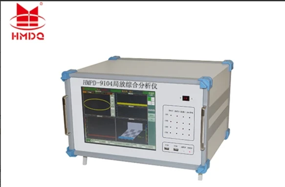
Figure 5 - The analysis end. Three simultaneous views of the same pulse train: the ellipse, the sequence and the three-dimensional pattern. Classification comes from reading them together, which is why the analysis layer, not the sensor, is where the last margin of reliability lives.

For Stage 1, the portable partial discharge detector range covers the survey work - acoustic emission, UHF, HF and transient earth voltage in one instrument, which is what makes a band-by-band background map at a live transformer practical in a single visit. The same manufacturer's PD-free test systems are the other half of the story: a laboratory reference at the factory is what makes the on-site baseline interpretable. SFRA and winding resistance measurement address the mechanical and connection failure modes PD monitoring does not cover, and transformer oil testing - including dissolved gas analysis - supplies the chemical evidence that a discharge has actually occurred. The PD test equipment category indexes the rest.

It will not give you a picocoulombs figure you can defend. Without a calibrated injection path, the level is an internal index, useful for trend on that asset and not comparable to a specification or to another transformer.

It will not see a defect that is dormant at the operating point. Online measurement has no voltage control. A defect that only becomes active under unusual load or temperature may be invisible until the condition recurs - which is an argument for correlating with load and temperature rather than for higher sensitivity.

It will not replace DGA. Online DGA tells you that the insulation has decomposed; PD monitoring tells you when, which phase, and roughly where. The two are complementary evidence, and a well-designed condition-monitoring scheme on a 220 kV transformer runs both.

It will not find a loose connection or a mechanical shift. Those are winding resistance and frequency-response measurements, on the same asset, on the same maintenance schedule.